Variational encoding(VAEs)

Problem setting

• Given a set of data points $D = ({x_i})_{i=1}^N$

• Where $x_i \in \mathbb{R}^d$ are iid samples from some unknown distribution $p_{\text{data}}$.

• We want to model $p_{\text{data}}$ as $p_{\theta}$ using a neural network.

• We model $p_{\theta}$ as a latent variable model

Modelling

Log likelihood is given by:

$$ \ell(\theta) = \log p_{\theta}(x) $$

We assume that each data point $x_i$ is associated with a latent variable $z_i$. Hence, we will introduce the latent variable $z$ and marginalize over it:

$$ \ell(\theta) = \log \sum_z p_{\theta}(x, z) $$

Let $q(z|x)$ be a conditional distribution over $z$ given $x$. We multiply and divide by $q(z|x)$ to get:

$$ \ell(\theta) = \log \sum_z q(z|x) \frac{p_{\theta}(x, z)}{q(z|x)} $$

This can be written as:

By Jensen’s inequality, we have:

Where $F_{\theta}(q)$ is the evidence lower bound (ELBO).

Here the first term is the conditional log likelihood of the data under the model. We want to maximise this term.

The second term is the KL divergence between the posterior and the prior. We want to minimise this term.

Variational Autoencoder

The Variational Autoencoder (VAE) architecture can be visualized as follows:

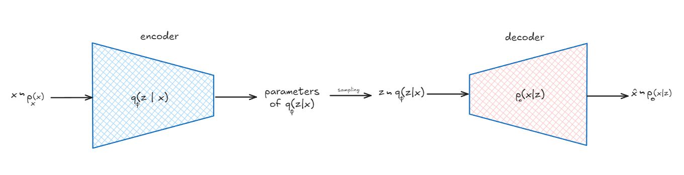
In this diagram, we can see the key components of a VAE:

• Encoder: We model $q(z|x)$ as a neural network with parameters $\phi$. The network takes in an observation $x$ and outputs the parameters of a Gaussian distribution ie mean $\mu_{\phi}(x)$ and covariance $\Sigma_{\phi}(x)$.

• Decoder: We model $p_{\theta}(x|z)$ as a neural network with parameters $\theta$. The network takes in a sampled latent variable $z$ from the distribution with parameters $\mu_{\phi}(x)$ and $\Sigma_{\phi}(x)$ and outputs a data sample $\hat{x}$. Post training, we use the decoder to generate new data samples ie works as generator.

Motivation for reparameterisation trick

Evidence is intractable, so we are optimizing a lower bound on it.

We need to be able to compute the gradient of the ELBO to be able to do gradient descent.

ELBO’s first term’s gradient is intractable because the sampling process is non-differentiable hence we use reparameterisation trick.

Reparameterisation trick

Recall that we have to minimize ELBO:

Focus on first term

We introduce a function $g_{\phi}(\epsilon)$ that transforms a noise variable $\epsilon$ into $z$

$$ z = g_{\phi}(\epsilon) $$

Where:

• $\epsilon \sim p(\epsilon)$ (typically a standard normal distribution)
• $g_{\phi}(\epsilon)$ is our reparameterization function typically $z=g_{\phi}(\epsilon) = \mu_{\phi}(x) + \sigma_{\phi}(x) \odot \epsilon$

This allows us to rewrite the expectation in terms of $\epsilon$

The gradient of the first term(required for backpropagation) can then be estimated using Monte Carlo sampling:

Reparameterisation trick in practice

In practice, the reparameterization trick is implemented as follows:

1. We pass a particulat data point $x_i$ through encoder network to get $\mu_{\phi}(x_i)$ and $\Sigma_{\phi}(x_i)$ which are the parameters of the distribution $q(z|x)$
2. We sample m number of $\epsilon_j$ from a standard normal distribution $N(0, 1)$ for $j = 1, \ldots, m$
3. We compute

for $j = 1, \ldots, m$, where $m$ is the number of latent variables we want to sample, and $\sigma_{\phi}(x_i) = \sqrt{\Sigma_{\phi}(x_i)}$ is the standard deviation. This gives us $m$ different $z_j^i$ values, each representing a point in the latent space.

4. We then pass each $z_j^i$ through the decoder network to get $m$ different data samples $\hat{x}_j^i$ where $j = 1, \ldots, m$.

5. We want to compute

• If we assume $p_{\theta}(x|z) = p_{\theta}(x|g_{\phi}(\epsilon)) \sim N(x; x_i, I)$, which is a model assumption. This allows us to calculate the log-likelihood $\log p_{\theta}(x|z)$ using the generated samples $\hat{x}_j^i$ and the original input $x_i$ as follows(derivation skipped):

• Alternatively, if we assume $p_{\theta}(x|z) = p_{\theta}(x|g_{\phi}(\epsilon))$ follows a Bernoulli distribution, which is often used for binary data, we can calculate the log-likelihood as follows:

Where:

• $x_i^t$ is the t-th dimension of the i-th input data point

• $\hat{x}_j^{i,t}$ is the t-th dimension of the j-th reconstructed sample for the i-th input

• T is the dimensionality of the input data

  This formulation is particularly useful for tasks like image generation where pixel values can be treated as binary (black or white) or probabilities of being active.

6. Propagate the gradient of the log-likelihood with respect to the model parameters $\theta$ to update the decoder network parameters.
7. Backpropagate through the encoder network to update its parameters $\phi$.

Second term of ELBO

Recall that:

the second term is:

$$ D_{KL} \left( q(z|x) \mid p_{\theta}(z) \right) $$

We want to minimise this term.

We assume the latent prior $p_\theta(z) \sim N(0, I)$, where $I$ is the identity matrix.

The approximate posterior $q(z|x)$ is modeled as $N(z; \mu_\phi(x), \Sigma_\phi(x))$.

Given these assumptions, we can derive the KL divergence in closed form as:

$$ D_{KL}(N(z; \mu_\phi(x), \Sigma_\phi(x)) | N(0, I)) = \frac{1}{2} \sum_{j=1}^J \left( \mu_{\phi,j}^2(x) + \Sigma_{\phi,j}(x) - \log \Sigma_{\phi,j}(x) - 1 \right) $$

Where:

• $J$ is the dimensionality of the latent space
• $\mu_{\phi,j}(x)$ is the j-th element of the mean vector
• $\Sigma_{\phi,j}(x)$ is the j-th diagonal element of the covariance matrix

Complete back propagation

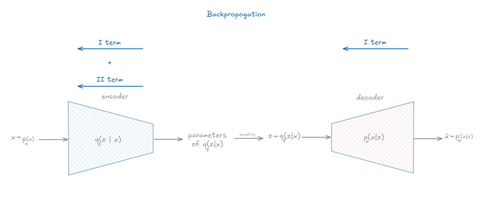
Here’s a step-by-step breakdown of the complete backpropagation process for a Variational Autoencoder (VAE):

1. Complete picture of passing $x_i$ through encoder
2. Get $\epsilon_i$
3. Get multiple $z$ … $z$
4. Pass all of them through decoder get $\hat{x}^1$ … $\hat{x}^m$
5. Train decoder using only first term
6. While training decoder, also train using second term

Inference

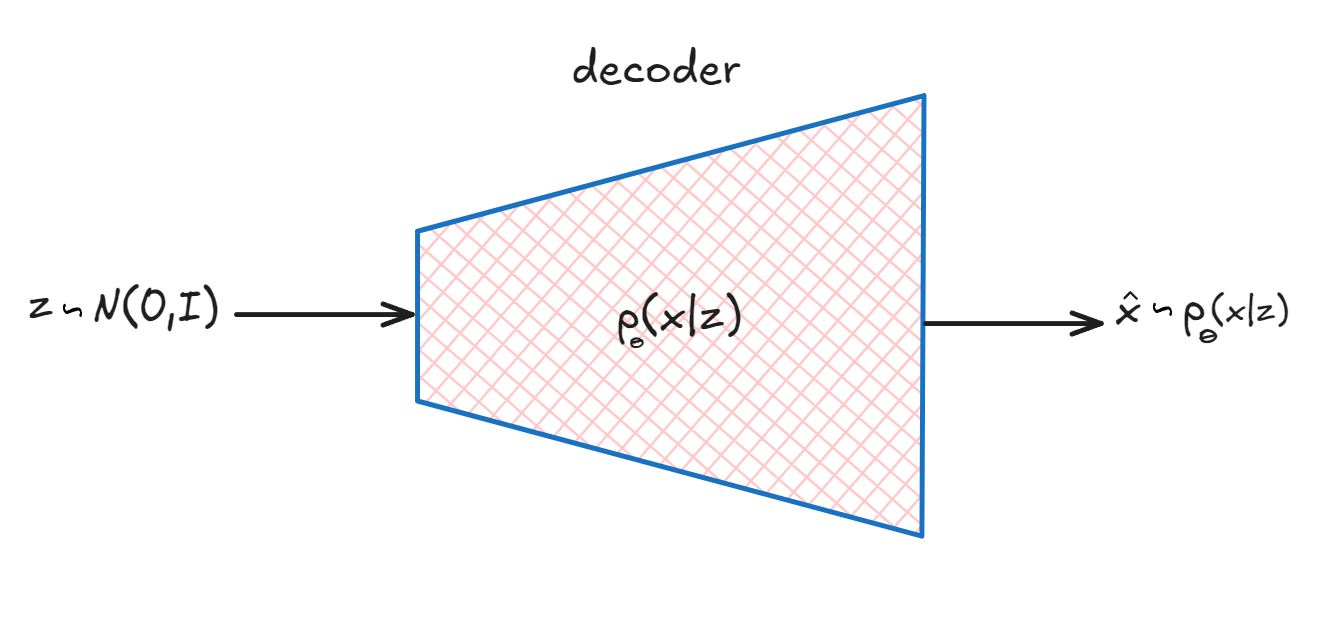
1. Sample from $N(0, I)$ to get $z$. This works because we trained the decoder wrt to the second term $D_{KL} \left( q(z|x) \mid p_{\theta}(z) \right)$
2. Pass $z$ through decoder to get $\hat{x}$