DDPM as special case of variational autoencoders (VAE)
Impose following structure on the VAE:
- Multiple latent variables, where each latent variable is associated with a timestep.
- Dim of all the latent variables is the same as the dim of the data.
- Assume a non learnable encoder unlike VAE where the encoder was learnable.
Notations
- $X_1, …, X_T$: Denote latent variables at different timesteps
- $p(X_0)$: Denote the model data distribution
- $X_{1:T} = (X_1, X_2, …, X_T)$: Denote the sequence of all latent variables
- $q(X_{1:T}|X_0)$: Denote the latent posterior
Latent posterior
Because $q(X_{1:T}|X_0)$ is not learnable, we need to define it - we make it first order markovian chain with gaussian transitions:
$$X_0 \rightarrow X_1 \rightarrow X_2 \rightarrow … \rightarrow X_T$$
This is also called encoding or forward process or adding noise process. Here:
$$X_t = \sqrt{\alpha_t} X_{t-1} + \sqrt{1-\alpha_t} \epsilon, \quad \epsilon \sim \mathcal{N}(0,I)$$
where $\alpha_t \in (0,1)$ called variance schedule are hyperparameters that control the variance of the latent variables at different timesteps. Generally, $\alpha_t$ is chosen to be a constant or a slowly decaying function of $t$ to ensure that the variance of the latent variables at different timesteps is not too high or too low.
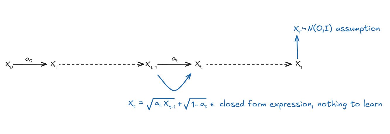
Because we are interested in modeling latents, we use the chain rule and Markov property of the forward process:
$$q(X_{1:T}|X_0) = \prod_{t=1}^T q(X_t|X_{t-1})$$
Because of reparameterization of $X_t = \sqrt{\alpha_t} X_{t-1} + \sqrt{1-\alpha_t} \epsilon, \quad \epsilon \sim \mathcal{N}(0,I)$
$$q(X_t|X_{t-1}) = \mathcal{N}(X_t; \sqrt{\alpha_t}X_{t-1}, (1-\alpha_t)I)$$
Model
We define model $p_\theta(X_0)$ as:
$$p_\theta(X_0) = \int p_\theta(X_{0:T}) , dX_{1:T}$$
However, this is not tractable to compute directly. Instead, we can use the Evidence Lower Bound (ELBO) to optimize our model.
Recall the Evidence Lower Bound (ELBO) in general is given by:
Hence,
The markov chain in reverse is also known as reverse/decoding/denoising/sampling process:
$$X_T \rightarrow X_{T-1} \rightarrow X_{T-2} \rightarrow … \rightarrow X_0$$
- It is also a first order markov chain with gaussian transitions
- Hence, we can express the modelled joint distribution of the reverse process by applying the chain rule of the reverse process:
$$p_\theta(X_{0:T}) = p(X_T) \prod_{t=1}^T p_\theta(X_{t-1}|X_t)$$
Where:
- $p(X_T)$ is the prior distribution of the latent variable at the final timestep
- $p_\theta(X_{t-1}|X_t)$ represents the transition probability from $X_{t-1}$ to $X_t$ in the reverse process, parameterized by $\theta$ which we aim to learn
Substitute $p_\theta(X_{0:T})$ in ELBO:
Using the Markov property of the forward process, we can rewrite $q(X_{1:T}|X_0)$ as:
$$ q(X_{1:T}|X_0) = \prod_{t=1}^T q(X_t|X_{t-1}) $$
Substituting this into the ELBO equation:
Breaking down the ELBO equation into components:
- First, we separate the log terms:
This gives us our final ELBO equation with three distinct terms:
- A reconstruction term: $\log p_\theta(X_0|X_1)$
- A prior matching term: $\log \frac{p(X_T)}{q(X_T|X_0)}$
- A transition matching term: $\sum_{t=2}^T \log \frac{p_\theta(X_{t-1}|X_t)}{q(X_{t-1}|X_t,X_0)}$