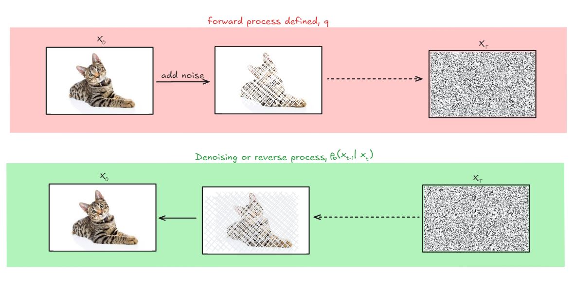
We were using latent variables $X_t$ to model the data as:
$$\log p_\theta(x_0) = \log \int p_\theta(x_{0:T}) dx_{1:T}$$
This formulation expresses the log-likelihood of the observed data $x_0$ as an integral over all possible latent variable sequences $x_{1:T}$. The model’s goal is to maximize this log-likelihood, which involves learning the parameters $\theta$ that define the generative process from $x_T$ back to $x_0$.
Also:
- $p_\theta(x_T) = \mathcal{N}(0, I)$ - The prior distribution of the final latent variable is a standard normal distribution
- $p_\theta(x_{0:T}) = p_\theta(x_T) \prod_{t=1}^T p_\theta(x_{t-1}|x_t)$ - The joint distribution of all latent variables is factorized using the chain rule
- $q(x_t|x_{t-1}) = \mathcal{N}(x_t; \sqrt{\alpha_t}x_{t-1}, (1-\alpha_t)I)$ - The forward process transition probability is a Gaussian distribution
- $q(x_{1:T}|x_0) = \prod_{t=1}^T q(x_t|x_{t-1})$ - The posterior of all latent variables given the data is factorized using the chain rule
Because the log likelihood is intractable, we constructed the ELBO of the model:
Reconstruction term
The reconstruction term is given by:
Recall that the forward process is defined as:
$$x_1 = \sqrt{\alpha_1} x_0 + \sqrt{1-\alpha_1} \epsilon, \quad \epsilon \sim \mathcal{N}(0,I)$$
To reconstruct $x_0$ from $x_1$ (the first latent sample), we assume a Gaussian distribution:
$$p_\theta(x_0|x_1) = \mathcal{N}(x_0; \mu_\theta(x_1, 1), \sigma_1^2 I)$$
Where:
- $\mu_\theta(x_1, 1)$ is the mean predicted by the model
- $\sigma_1^2$ is a fixed variance (usually set to $\beta_1 = 1 - \alpha_1$)
With this Gaussian assumption, the reconstruction term becomes:
Prior matching term
The prior matching term is given by:
Because the term inside the expectation is independent of $x_{2:T}$, we can simplify it to $\mathbb{E}_{q(x_T |x_0)}$
$$T_2 = - D_{KL}(q(x_T|x_0) | p_\theta(x_T))$$
Note that $T_2$ can be ignored during optimization because:
- It doesn’t depend on the model parameters $\theta$
- $p_\theta(x_T) = \mathcal{N}(0, I)$ is fixed
This prior matching term is similar to the KL divergence term in Variational Autoencoders (VAEs), $D_{KL}(q(z|x) | p(z))$, where it encourages the approximate posterior to match the prior distribution.
Transition matching/ Consistency/ Denoising matching term
The transition matching term is given by:
It can be shown that:
Consider the first term in the KL divergence. By applying Bayes’ law, we can rewrite it as:
$$q(x_{t-1}|x_t,x_0) = q(x_t|x_{t-1},x_0) \frac{q(x_{t-1}|x_0)}{q(x_t|x_0)}$$
$$q(x_{t-1}|x_t,x_0) = \frac{q(x_t|x_{t-1})q(x_{t-1}|x_0)}{q(x_t|x_0)}$$
We know that:
- $q(x_t|x_{t-1}) = \mathcal{N}(x_t; \sqrt{\alpha_t}x_{t-1}, (1-\alpha_t)I)$
- $q(x_t|x_0) = \mathcal{N}(x_t; \sqrt{\bar{\alpha}_t}x_0, (1-\bar{\alpha}_t)I)$ where $\bar{\alpha}t = \prod{i=1}^t \alpha_i$ - Skipped derivation but it is in class notes
- $q(x_{t-1}|x_0) = \mathcal{N}(x_{t-1}; \sqrt{\bar{\alpha}{t-1}}x_0, (1-\bar{\alpha}{t-1})I)$
Substituting these into the equation for $q(x_{t-1}|x_t,x_0)$, we get(Derivation skipped but it is eqn 84 in https://arxiv.org/pdf/2208.11970 ):
$$q(x_{t-1}|x_t,x_0) = \mathcal{N}(x_{t-1}; \mu_q(x_t,x_0), \Sigma_q(t))$$
Where:
Now, let’s consider the second term in the KL divergence, $p_\theta(x_{t-1}|x_t)$. In DDPM, this is modeled as a Gaussian distribution:
$$p_\theta(x_{t-1}|x_t) = \mathcal{N}(x_{t-1}; \mu_\theta(x_t), \Sigma_\theta(x_t))$$
The KL divergence between two Gaussian distributions has a closed-form expression. Therefore, we can compute $T_3$ analytically:
Here, $d$ is the dimensionality of the data, and $tr$ denotes the trace of a matrix.
This term encourages the learned reverse process $p_\theta(x_{t-1}|x_t)$ to match the true posterior $q(x_{t-1}|x_t,x_0)$, which is why it’s called the transition matching or consistency term.