Denoising Diffusion Probabilistic Models (DDPM) - part 3

Recall that:

Here:

• $q(x_{t-1}|x_t,x_0)$ is the noising distribution after applying the forward process for $t-1$ steps
• $p_\theta(x_{t-1}|x_t)$ is the model’s predicted denoising distribution after applying the reverse process

We also know that:

$$q(x_{t-1}|x_t,x_0) = \mathcal{N}(x_{t-1}; \mu_q(x_t,x_0), \Sigma_q(t))$$

where $\mu_q(x_t,x_0)$ and $\Sigma_q(t)$ are the mean and covariance of the posterior distribution and:

The covariance $\Sigma_q(t)$ is given by:

$$ \Sigma_q(t) = \frac{(1-\alpha_t)(1-\bar{\alpha}_{t-1})}{1-\bar{\alpha}_t}I = \sigma_q^2(t) I $$

where $\sigma_q^2(t)$ is a scalar that depends on $t$. This is a model assumption that simplifies the calculations by assuming $\Sigma_q(t)$ is a diagonal matrix (proportional to the identity matrix $I$) for each timestep $t$, with its elements determined by $\sigma_q^2(t)$.

Also, we have:

$$p_\theta(x_{t-1}|x_t) = \mathcal{N}(x_{t-1}; \mu_\theta(x_t, t), \sigma_\theta^2 I)$$

where $\mu_\theta(x_t, t)$ is the mean of the model’s prediction and $\sigma_\theta^2$ is a scalar variance, assuming the covariance is proportional to the identity matrix $I$.

Note: In both the forward process ($q$) and the reverse process ($p$), the covariance matrices are assumed to be diagonal and proportional to the identity matrix. This simplification is indeed a key assumption in the DDPM model.

Hence:

$$T_3 = - \sum_{t=2}^T \mathbb{E}_{q(x_t|x_0)} [\frac{1}{2\sigma_\theta^2} ||\mu_q(x_t,x_0) - \mu_\theta(x_t, t)||^2]$$

Notice that:

• $\mu_q(x_t,x_0)$ is the mean of the posterior distribution, which is a function of $x_t$ and $x_0$. This is a known value.
• $\mu_\theta(x_t, t)$ is the mean of the model’s prediction, which is a function of $x_t$ and $t$. This is a learnable parameter.

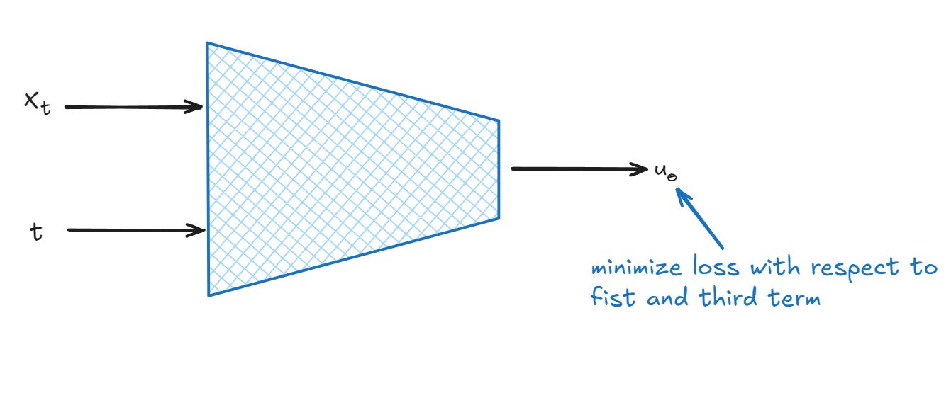
This could tatally work however the loss is formulated by reparametrizing.

Reparameterization

Recall that the forward process is defined as:

$$x_t = \sqrt{\bar{\alpha}_t} x_0 + \sqrt{1-\bar{\alpha}_t} \epsilon, \quad \epsilon \sim \mathcal{N}(0, I)$$

From this, we can rearrange to express $x_0$ in terms of $x_t$:

$$x_0 = \frac{x_t - \sqrt{1-\bar{\alpha}_t} \epsilon}{\sqrt{\bar{\alpha}_t}}$$

Substituting this expression for $x_0$ into the equation for $\mu_q(x_t, x_0)$, we get:

Simplifying, we have:

$$\mu_q(x_t, x_0) = \frac{1}{\sqrt{\bar{\alpha}_t}} x_t - \frac{(1-\alpha_t)}{\sqrt{1-\bar{\alpha}_t} \sqrt{\bar{\alpha}_t}} \epsilon$$

Note that this is a known value.

Also we can write $\mu_\theta(x_t, t)$ as:

where $\epsilon_\theta(x_t, t)$ is the model's prediction for the noise at time step $t$. This can be done because we can always reparametrize one Gaussian distribution to another Gaussian distribution.

Instead of learning $\mu_\theta(x_t, t)$(learn to predict the noise), we learn $\epsilon_\theta(x_t, t)$ and then use the above equation to get $\mu_\theta(x_t, t)$.

Now substitute $\mu_q(x_t, x_0)$ and $\mu_\theta(x_t, t)$ into $T_3$ we get:

Simplifying the expression inside the norm, we get:This can be further simplified to:Finally, we can express the proportionality:## Architecture

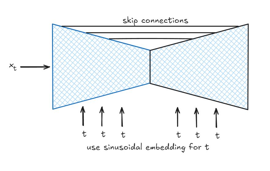
We do not give a scalar $t$ to the network because the network will simply ignore it, hence we give time using sinusoidal embedding. The time embedding is concatenated with the residual path as:

Training

The training process for DDPM involves the following steps:

1. Sample a random data point: Select a data point $x_0$ from the training dataset.

2. Sample a random time step: Choose a random time step $t$ from a uniform distribution over the range $[1, T]$.

3. Sample noise: Generate a noise sample $\epsilon \sim \mathcal{N}(0, I)$.

4. Generate noisy data: Create the noisy data $x_t$ using the forward process equation: $$x_t = \sqrt{\bar{\alpha}_t} x_0 + \sqrt{1 - \bar{\alpha}_t} \epsilon$$

5. Predict the noise: Use the model to predict the noise $\epsilon_\theta(x_t, t)$ at time step $t$.

6. Compute the loss: Calculate the loss as the mean squared error between the true noise $\epsilon$ and the predicted noise $\epsilon_\theta(x_t, t)$: $$L_t = \left| \epsilon - \epsilon_\theta(x_t, t) \right|_2^2$$

7. Backpropagation: Perform backpropagation to compute the gradients of the loss with respect to the model parameters.

8. Update the model parameters: Use an optimizer (e.g., Adam) to update the model parameters based on the computed gradients.

9. Repeat: Iterate through the training dataset and repeat the above steps for a fixed number of epochs or until convergence.

By following these steps, the model learns to predict the noise at each time step, which can then be used to generate new samples by reversing the diffusion process.

Inference

The inference process in DDPM involves reversing the diffusion process to generate new samples. The steps are as follows:

1. Sample from the prior: Start by sampling $x_T \sim \mathcal{N}(0, I)$, which is the prior distribution.

2. Reverse the diffusion process: Sequentially sample $x_{t-1}$ from $x_t$ for $t = T, T-1, \ldots, 1$ using the learned reverse process $p_\theta(x_{t-1}|x_t)$.

   The reverse process is defined as: $x_T$ to $x_0$ through intermediate steps $x_{T-1}, \ldots, x_1$.

where $z \sim \mathcal{N}(0, I)$ if $t > 1$, and $z = 0$ if $t = 1$ and $\sigma_t^2 = \beta_t = \frac{1-\bar{\alpha}_{t-1}}{1-\bar{\alpha}_t} \cdot (1-\alpha_t)$.

3. Obtain the final sample: The final sample $x_0$ is obtained after completing the reverse process.