Recap
- $J_{ESM}(\theta) = \mathbb{E}_{p(x)} \left[ \frac{1}{2} | \hat{s}(x; \theta) - \nabla_x \log p(x) |^2 \right]$
- $J_{ISM}(\theta) = \mathbb{E}_{p(x)} \left[ \frac{1}{2} | \hat{s}(x; \theta) |^2 + \text{tr}(\nabla_x \hat{s}(x; \theta)) \right] + C$
- Theorem: $J_{ISM}(\theta) = J_{ESM}(\theta) + C$
- $\theta^* = \mathop{\arg \min}_{\theta} J_{ISM}(\theta)$
- $x_{t+1} = x_t + \alpha \cdot \hat{s}(x_t; \theta^*) + \sqrt{2\alpha} \epsilon, \quad \epsilon \sim \mathcal{N}(0, I)$
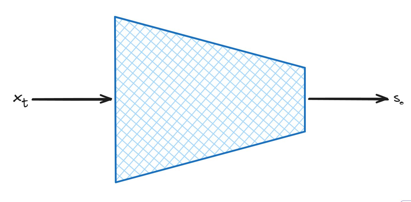
- $\hat{s}(x; \theta)$ modelled using a neural network
There is a problem with calculating the trace term
The implicit score matching loss function, as we discussed earlier, is given by:
$$J_{ISM}(\theta) = \mathbb{E}_{p(x)} \left[ \frac{1}{2} | \hat{s}(x; \theta) |^2 + \text{tr}(\nabla_x \hat{s}(x; \theta)) \right] + C$$
However, there’s a significant challenge in calculating this loss function, particularly with the trace term:
$$\text{tr}(\nabla_x \hat{s}(x; \theta))$$
The problem arises because:
- $\nabla_x \hat{s}(x; \theta)$ is the Hessian of $\log p(x)$ with respect to the input $x$.
- For high-dimensional data (which is common in many applications), this Hessian becomes extremely large.
- Computing the trace of this large Hessian matrix is computationally expensive and often intractable.
This computational challenge motivates the need for alternative approaches to score matching, which we’ll explore in the following sections.
Projected score matching
Projected score matching is a technique that involves projecting the score function onto a lower-dimensional subspace.
The projected score matching loss function can be expressed as:
Where:
- $\hat{s}_\theta(x)$ is the estimated score function
- $s(x)$ is the true score function
- $v$ is a random projection vector
This formulation allows us to estimate the score function without explicitly computing the trace of the Hessian, which is computationally expensive in high-dimensional spaces. Instead, we project the score function onto random vectors $v$, effectively reducing the dimensionality of the problem.
However this cannot be computed(similar to the problem with calculating $J_{ISM}$) because we do not know $s(x)$
Hence we need to find an alternative way to compute the loss function which leads us to sliced score matching
Sliced Score Matching
The SSM loss function can be expressed as:
Key aspects of Sliced Score Matching:
Random Projections: Like projected score matching, SSM uses random projections to reduce dimensionality. However, SSM specifically uses unit vectors sampled from a uniform distribution on the unit sphere.
Efficient Computation: The second term $v^\top (\nabla_x \hat{s}_\theta(x)) v$ can be computed efficiently using automatic differentiation, avoiding the need to explicitly calculate the full Hessian matrix.
Theorm
The relationship between Projected Score Matching (PSM) and Sliced Score Matching (SSM) can be expressed through the following theorem:
$$J_{PSM}(\theta) = J_{SSM}(\theta) + C$$
Where:
- $J_{PSM}(\theta)$ is the loss function for Projected Score Matching
- $J_{SSM}(\theta)$ is the loss function for Sliced Score Matching
- $C$ is a constant term independent of $\theta$
Following assumptions were made to prove the theorem:
A1. $p(x)$ and $s(x)$ are differentiable
A2:
A3. $\lim_{|x| \to \infty} p(x)\hat{s}(x; \theta) = 0$ for any $\theta$
A4:
This theorem demonstrates that under certain conditions, optimizing the SSM objective is equivalent to optimizing the PSM objective, up to a constant difference. This relationship provides a theoretical foundation for the use of Sliced Score Matching as an efficient alternative to Projected Score Matching.
How to compute $J_{SSM}$
$J_{SSM}$ can be computed using Monte Carlo estimates. Given a datapoint ${x_i}$ take $m$ projections and approximate the SSM loss function as follows:
This Monte Carlo approximation allows us to practically compute the SSM loss using a finite number of data samples and random projections, making it feasible for optimization in machine learning models.