Recap
- Langevin equation: $x_{t+1} = x_t + \alpha \cdot \nabla_x \log p(x_t) + \sqrt{2\alpha} \epsilon, \quad \epsilon \sim \mathcal{N}(0, I)$
- score function: $\nabla_x \log p(x) = s(x)$
- $J_{ESM}(\theta) = \mathbb{E}_{p(x)} \left[ \frac{1}{2} | \hat{s}(x; \theta) - \nabla_x \log p(x) |^2 \right]$
- $J_{ISM}(\theta) = \mathbb{E}_{p(x)} \left[ \frac{1}{2} | \hat{s}(x; \theta) |^2 + \text{tr}(\nabla_x \hat{s}(x; \theta)) \right] + C$
- Theorem: $J_{ISM}(\theta) = J_{ESM}(\theta) + C$
- $J_{PSM}(\theta) = \frac{1}{2} \mathbb{E}_v \mathbb{E}_{p(x)} \left[ \| v^\top \hat{s}_\theta(x) - v^\top s(x) \|^2 \right]$
- $J_{SSM}(\theta) = \mathbb{E}_v \mathbb{E}_{p(x)} \left[ \frac{1}{2}(v^\top \hat{s}_\theta(x))^2 + v^\top (\nabla_x \hat{s}_\theta(x)) v \right]$
- Theorem: $J_{PSM}(\theta) = J_{SSM}(\theta) + C$
Big picture plan
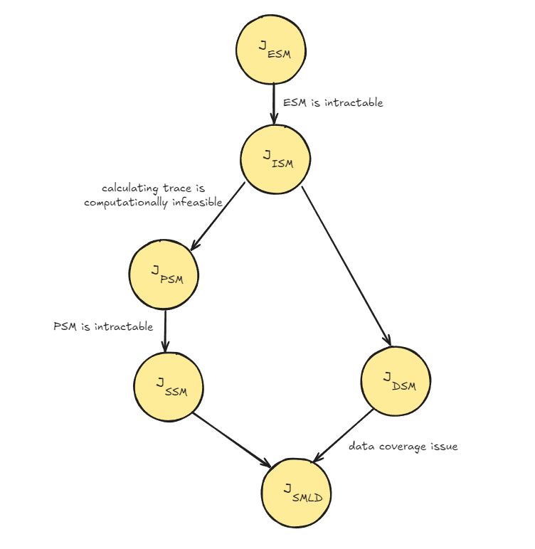
Denoising score matching
Denoising score matching (DSM) is an alternative approach to score matching. It introduces an auxiliary variable and works with conditional scores, which offers several advantages.
Let’s start with the DSM objective:
The DSM objective allows us to learn the score function $\nabla_x \log p(x)$ by:
- Generating training pairs $(x,x’)$ by adding noise to data samples
- Leveraging the known form of $p(x|x’)$ for Gaussian noise
- Avoiding direct computation of the intractable normalization constant
Key aspects of Denoising Score Matching:
Auxiliary Variable: DSM introduces $x’$, which is a noisy version of the original data point $x$. This allows us to work with conditional distributions.
Conditional Score: Instead of estimating the score of the data distribution directly, DSM estimates the conditional score $\nabla_{x} \log p(x|x’)$.
Gaussian Noise: Typically, Gaussian noise is added to create $x’$. This has two significant benefits:
- We can add Gaussian noise to our data easily.
- The conditional distribution $p(x|x’)$ becomes Gaussian, which has a known analytical form for its score.
Theorem: There’s an important relationship between DSM and the original score matching objective:
$$J_{ESM}(\theta) = J_{DSM}(\theta) + C$$
Where $C$ is a constant independent of $\theta$. This theorem shows that optimizing the DSM objective is equivalent to optimizing the original score matching objective.
The benefits of using conditional scores and Gaussian noise make DSM a powerful and practical approach to score matching, addressing many of the computational challenges faced by earlier methods.
Continue DSM
Let’s continue exploring Denoising Score Matching (DSM) in more detail. The original DSM objective was:
This gives us:
Score of Perturbation Kernel: The term $\nabla_{\tilde{x}} \log q_\sigma(\tilde{x}|x)$ can be derived analytically:
$$\begin{aligned} \nabla_{\tilde{x}} \log q_\sigma(\tilde{x}|x) &= -\nabla_{\tilde{x}} \frac{(\tilde{x}-x)^2}{2\sigma^2} \ &= -\frac{\tilde{x}-x}{\sigma^2} \end{aligned}$$
Substituting this back into our objective:
Reparameterization for Efficient Training
We can make this objective more computationally tractable through reparameterization. Instead of sampling $\tilde{x}$ directly, we express it in terms of $x$ and $\epsilon$:
$$\tilde{x} = x + \sigma\epsilon, \quad \epsilon \sim \mathcal{N}(0, I)$$
This transforms our objective into:
Critical Properties of this Formulation:
Scale-Aware Training: The $\frac{1}{2\sigma^2}$ factor naturally weights the loss more heavily at smaller noise levels. This ensures accurate denoising across different scales.
Direct Noise Prediction: Instead of predicting scores, the model learns to predict the noise directly.
Data Coverage Problem
A fundamental challenge in score matching is ensuring accurate score estimation across the entire data distribution $p(x)$, particularly in regions of low density. This is known as the data coverage problem.
Noise Conditional Score Networks (NCSNs) address this challenge through a multi-scale approach:
Noise Scale Hierarchy: $${\sigma_i}_{i=1}^L, \quad \text{where } \sigma_1 < \sigma_2 < … < \sigma_L$$
- $L$ typically ranges from 10 to several hundred scales
- $\sigma_1 = \sigma_{min}$ (minimal noise)
- $\sigma_L = \sigma_{max}$ (maximal noise)
Distribution Bridging: Two key conditions are enforced:
- $p_{\sigma_{min}}(x) \approx p(x)$ (preserves original distribution)
- $p_{\sigma_{max}}(x) \approx \mathcal{N}(0, I)$ (approaches Gaussian)
Noise Application: For each scale $\sigma_i$: $$p_{\sigma_i}(\tilde{x}|x) = \mathcal{N}(\tilde{x}|x, \sigma_i^2I)$$
Score Estimation: The model learns scale-conditional scores: $$s_\theta(x, \sigma_i) \approx \nabla_x \log p_{\sigma_i}(x)$$
Scale-Specific Loss:
- Combined Training Objective:
Benefits of this Multi-Scale Approach:
Comprehensive Coverage:
- High-density regions: Accurate modeling with small $\sigma_i$
- Low-density regions: Stable estimation with large $\sigma_i$
Smooth Interpolation:
- Gradual transition between noise levels
- Continuous coverage of the data manifold
Training Stability:
- Different scales provide complementary learning signals
- Reduced sensitivity to individual scale choices
This approach enables NCSNs to effectively model complex data distributions while maintaining stability and accuracy across all regions of the data space.