Big picture of what we are going to do:
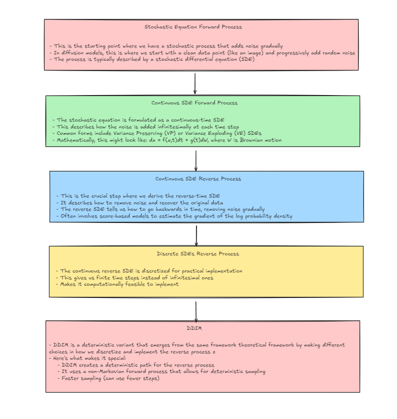
Big picture of SDEs
This topic comes under stochastic calculus, which deals with functions whose derivatives yield random vectors rather than deterministic points.
In traditional calculus, when we take the derivative of a function at a point, we get a fixed value ie a scalar that represents the instantaneous rate of change. However, in stochastic calculus, the derivative at any point is a random variable.
Formal definition of SDEs
Now let’s understand the formal definition of SDEs:
An Ordinary Differential Equation (ODE) can be written as: $$\frac{dx(t)}{dt} = f(x,t)$$ or in differential form: $$dx = f(x,t)dt$$
A Stochastic Differential Equation (SDE) adds a noise term: $$\frac{dx(t)}{dt} = f(x,t) + g(x,t)dW(t)$$ or in differential form: $$dx = f(x,t)dt + g(x,t)dB_t$$
where:
- $f(x,t)$ is called the drift term (deterministic component that describes the average behavior)
- $g(x,t)$ is called the diffusion term (controls the magnitude of random fluctuations)
- $W(t)$ is a Wiener process (Brownian noise) - a continuous-time stochastic process
- $B_t$ is a Brownian motion, $dB_t$ is the increment of Brownian motion where $$dB_t \sim N(0,dt)$$ $$dB_t = \sqrt{dt}\epsilon \quad \text{where} \quad \epsilon \sim N(0,1)$$
Key points about SDEs:
- An ODE is a special case where $g(x,t) = 0$
- The SDE is a stochastic process
We can define important properties of an SDE:
Mean/drift: $$m(t) = \mathbb{E}[x(t)] \leftarrow f(x,t)$$
Variance: $$v(t) = \text{Var}(x(t)) \leftarrow g(x,t)$$
This provides one way to analyze and understand SDEs.
Brownian Motion definition
A standard Brownian Motion (BM) is a random process $X = {X_t : t \in [0,\infty)}$ with state space $\mathbb{R}$ ie $X_t \in \mathbb{R}$ that satisfies the following properties:
$X_0 = 0$ with probability 1
- The process always starts at zero
Has stationary increments:
- For any $t \in [0,\infty)$, the distribution of $X_t - X_s$ only depends on the time difference $(t-s)$
- The behavior of changes doesn’t depend on when we start observing
Has independent increments:
- For any times $t_1 < t_2 < … < t_n \in [0,\infty)$
- The increments $X_{t_2} - X_{t_1}, X_{t_3} - X_{t_2}, …, X_{t_n} - X_{t_{n-1}}$ are independent
- For any non-overlapping time intervals
- What happens in one time period doesn’t affect what happens in another
For any $t \in [0,\infty)$: $X_t \sim \mathcal{N}(0,t)$ (Normal distribution with mean 0 and variance t)
- The position at any time follows a normal distribution with variance growing linearly with time
With probability 1, $t \mapsto X_t$ is continuous on $[0,\infty)$
- The path is continuous - no sudden jumps
Out of the above properties, we will use only the following:
- $X_t - X_s \sim \mathcal{N}(0,t-s)$
- The change over any interval follows a normal distribution
- $X_t \sim \mathcal{N}(0,t)$
- The position at any time follows a normal distribution
- $X_{t+s} - X_s \perp X_s$ (independence of increments)
- Future changes are independent of current position
Lets talk about $B_t$ - What it is not
Let’s consider how Brownian motion behaves when we look at small time intervals:
Consider $B_{t+h} - B_t$ where:
- $h > 0$: Looking at a small time step
- $B_{t+h} - B_t \sim B_h$ (from stationarity)
- $h < 0$: $B_{t+h} - B_t \sim -B_{-h}$ (from symmetry)
When we combine both: $B_{t+h} - B_t \sim B_{|h|}$
Therefore: $\frac{B_{t+h} - B_t}{h} \sim \mathcal{N}(0,{|h|})$
$$\frac{B_{t+h} - B_t}{h} \sim \frac{1}{h}\mathcal{N}(0,|h|) = \mathcal{N}(0,\frac{1}{h})$$
Therefore, the variance is: $$\text{Var}(\frac{B_{t+h} - B_t}{h}) = \text{Var}(\frac{1}{h}B_{|h|}) = \frac{1}{h^2}\text{Var}(B_{|h|}) = \frac{1}{h^2}|h| = \frac{1}{h}$$
Taking the limit as h approaches 0: $$\lim_{h \to 0} \text{Var}(\frac{B_{t+h} - B_t}{h}) = \lim_{h \to 0} \frac{1}{h} = \infty$$
Theorem: With probability 1, Brownian motion $B_t$ is nowhere differentiable on $[0,\infty)$.
This means that Brownian motion is not differentiable this is because:
- The variance of the rate of change becomes infinite as we look at smaller time intervals
- This means the rate of change becomes arbitrarily large and fluctuates wildly
- No well-defined derivative can exist under these conditions
Hence, $\frac{B_{t+h} - B_t}{h}$ does not converge in distribution (weakest form of convergence).
Lets talk about $B_t$ - What it is
While we cannot directly talk about the derivative of $B_t$ (since Brownian motion is not differentiable in the classical sense), we can still analyze it in terms of finite differences and perturbations.
Let’s define a perturbation $W_t^\epsilon$ as:
$$W_t^\epsilon = \frac{B_{t+\epsilon} - B_t}{\epsilon}$$
where $\epsilon$ represents a small time increment.
Now, consider the limit as $\epsilon \to 0$:
$$W_t = \lim_{\epsilon \to 0} W_t^\epsilon = \lim_{\epsilon \to 0} \frac{B_{t+\epsilon} - B_t}{\epsilon}$$
However, since $B_t$ is nowhere differentiable, $W_t$ does not exist in the usual sense. Instead, this expression can be interpreted in a distributional sense, often written informally as:
$$W_t \stackrel{\Delta}{=} \frac{dB_t}{dt}$$
Understanding the “White Noise” Process Note: This is an abuse of notation since $B_t$ is not differentiable. Instead, $W_t$ represents what we call white noise, which can be thought of as the “derivative” of Brownian motion in a generalized sense.
White noise, $W_t$, is a random process with constant power spectral density and is formally characterized by:
$$W_t \sim \frac{1}{\sqrt{dt}} \cdot \mathcal{N}(0,1)$$
This scaling factor $\frac{1}{\sqrt{dt}}$ ensures that the variance of $W_t$ scales inversely with the time increment $dt$, making its variance effectively infinite as $dt \to 0$ — a key property of white noise.
Increment Representation of Brownian Motion Using this notion of white noise, we can more rigorously express the increment of Brownian motion $B_t$ over a small interval $dt$ as:
$$dB_t = \sqrt{dt} \cdot \epsilon, \quad \epsilon \sim \mathcal{N}(0,1)$$
This expression indicates that the increment $dB_t$ over a tiny interval $dt$ behaves like a normal random variable with mean $0$ and variance $dt$.
This understanding forms the basis for Itô calculus, where these infinitesimal increments $dB_t$ are used to define stochastic integrals and develop a calculus for non-differentiable processes.