Motivation for state space models
- RNNs can handle variable length inputs however they are not parallelizable.
- CNNs are parallelizable however they cannot handle variable length inputs.
Can we get the best of both worlds?
Linear State Space Models
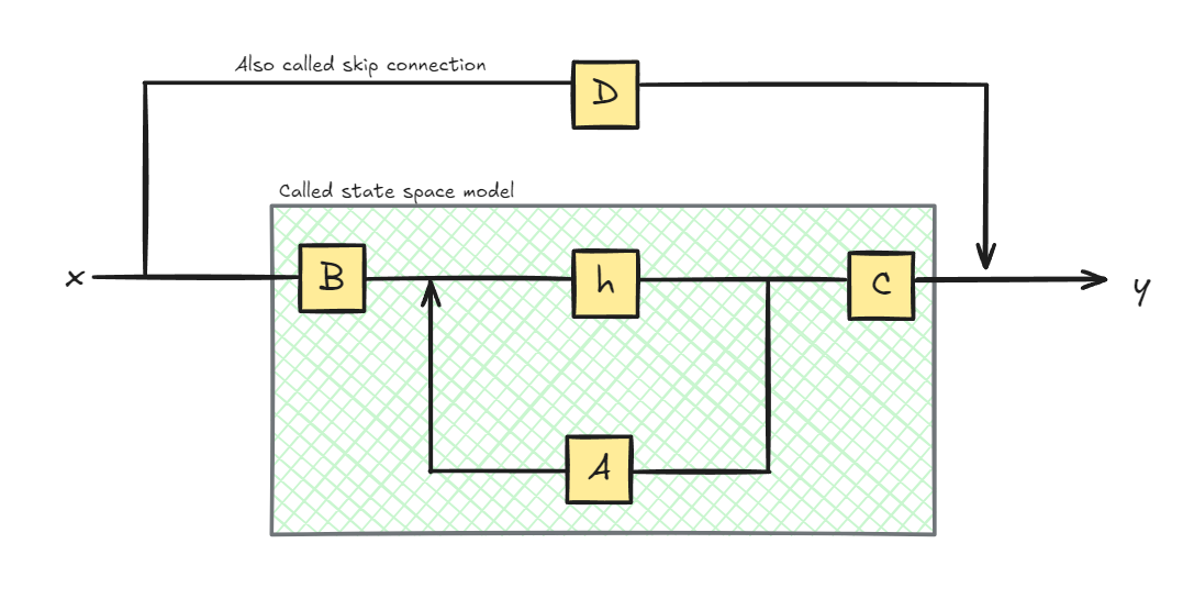
A linear state space model consists of two equations:
$$h’(t) = Ah(t) + Bx(t)$$ $$y(t) = Ch(t) + Dx(t)$$
where:
- $h(t)$ is the hidden state at time $t$
- $x(t)$ is the input at time $t$
- $y(t)$ is the output at time $t$
- $h’(t)$ is the derivative of the hidden state with respect to time
- $A, B, C, D$ are learnable parameter matrices that define the dynamics
The first equation describes how the hidden state evolves over time based on:
- The current hidden state $Ah(t)$ term
- The current input $Bx(t)$ term
The second equation describes how the output is generated from:
The current hidden state $Ch(t)$ term
The current input $Dx(t)$ term
Euler’s method
One common way to solve these equations numerically is using Euler’s method. Given a small time step $\Delta t$, we can approximate the derivative as:
$$\frac{dh(t)}{dt} \approx \frac{h(t+\Delta t) - h(t)}{\Delta t}$$
This approximation comes from the definition of a derivative as the limit of a difference quotient. Rearranging this gives us the forward Euler update rule:
$$h(t + \Delta t) \approx h(t) + \Delta t \cdot h’(t)$$
Substituting in the state equation $h’(t) = Ah(t) + Bx(t)$:
$$h(t + \Delta t) \approx h(t) + \Delta t \cdot (Ah(t) + Bx(t))$$ $$= h(t) + \Delta t \cdot Ah(t) + \Delta t \cdot Bx(t)$$ $$= (I + \Delta t A)h(t) + \Delta t Bx(t)$$
Where $I$ is the identity matrix. This gives us a discrete-time update rule that we can implement efficiently. The accuracy of this approximation depends on the time step $\Delta t$ - smaller steps yield better accuracy but require more computational steps. This tradeoff between accuracy and computational efficiency is a key consideration when implementing these models.
Now, we can rewrite this using discrete time notation where $t$ represents time steps: Let $h(t + \Delta t) = h_t$ and $h(t) = h_{t-1}$ Let $\bar{A} = (I + \Delta t A)$ and $\bar{B} = \Delta t B$
This gives us: $$h_t = \bar{A}h_{t-1} + \bar{B}x_t$$
The second equation doesn’t involve derivatives, so it simply becomes: $$y_t = Ch_t + Dx_t$$
where:
- $t \in {t_1, t_2, …, t_k}$ represents discrete time steps
- $\bar{A} = (I + \Delta t A)$ is the discretized state transition matrix
- $\bar{B} = \Delta t B$ is the discretized input matrix
- $h_t$ is the hidden state vector at discrete time step $t$
- $x_t$ is the input vector at time step $t$
- $y_t$ is the output vector at time step $t$
Unrolling the equations
Let’s assume initial state $h_{-1} = 0$. Then:
$$h_0 = \bar{B}x_0$$ $$y_0 = Ch_0 = C\bar{B}x_0$$
Now lets assume $D=0$. Then:
$$h_1 = \bar{A}h_0 + \bar{B}x_1 = \bar{A}\bar{B}x_0 + \bar{B}x_1$$ $$y_1 = Ch_1 = C(\bar{A}\bar{B}x_0 + \bar{B}x_1)$$
Similarly:
$$h_2 = \bar{A}h_1 + \bar{B}x_2 = \bar{A}^2\bar{B}x_0 + \bar{A}\bar{B}x_1 + \bar{B}x_2$$ $$y_2 = Ch_2 = C(\bar{A}^2\bar{B}x_0 + \bar{A}\bar{B}x_1 + \bar{B}x_2)$$
And in general, for any time step $k$:
$$h_k = \bar{A}^k\bar{B}x_0 + \bar{A}^{k-1}\bar{B}x_1 + … + \bar{A}\bar{B}x_{k-1} + \bar{B}x_k$$ $$y_k = Ch_k = \sum_{i=0}^k C\bar{A}^{k-i}\bar{B}x_i$$
where we define $\bar{A}^0 = I$ (identity matrix).
The matrix part of $y_k$ is called the convolution kernel of the state space model: $$K = [C\bar{B}, C\bar{A}\bar{B}, C\bar{A}^2\bar{B}, …]$$
A major benefit of representing the SSM as a convolution is that it can be trained in parallel like Convolutional Neural Networks (CNNs). However, due to the fixed kernel size, their inference is not as fast and unbounded as RNNs.
Initialization of A matrix
Matrix A is initialized using HiPPO for High-order Polynomial Projection Operators. The HiPPO matrix A is defined as follows:
For an $N$ x $N$ matrix $A$, the entries $A[n,k]$ are:
For entries below the diagonal ($n > k$): $$A[n,k] = ((2n + 1)^{1/2} \cdot (2k + 1)^{1/2})$$
For entries on the diagonal ($n = k$): $$A[n,k] = n + 1$$
For entries above the diagonal ($n < k$): $$A[n,k] = 0$$
Building matrix A using HiPPO was shown to be much better than initializing it as a random matrix. The idea behind the HiPPO Matrix is that it produces a hidden state that memorizes its history. Mathematically, it does so by tracking the coefficients of a Legendre polynomial which allows it to approximate all of the previous history.
A problem
If $\bar{A}$ is not diagonalizable, then we cannot compute $\bar{A}^k$ efficiently. Hence it is written as: $$\bar{A} = \Lambda + P\beta^H$$
where:
- $\Lambda$ is a diagonal matrix
- $P$ is a low rank matrix
- $\beta^H$ is the conjugate transpose of some vector $\beta$
To compute powers efficiently, we can:
- Transform the matrix to the inverse Fourier domain
- Compute the powers in the inverse Fourier domain
- Transform the result back to the time domain
This allows computation in linear time rather than having to explicitly calculate matrix powers.
Linear Time Invariance
Recall that: $$y_k = Ch_k = \sum_{i=0}^k C\bar{A}^{k-i}\bar{B}x_i$$ These representations share an important property, namely that of Linear Time Invariance (LTI). LTI states that the SSMs parameters, A, B, and C, are fixed for all timesteps. This means that matrices A, B, and C are the same for every token the SSM generates.
In other words, regardless of what sequence you give the SSM, the values of A, B, and C remain the same. We have a static representation that is not content-aware.
Mamba
Mamba is a state space model that addresses the limitations of Linear Time Invariance (LTI) through several key innovations:
- Recurrent State Space Model: The continuous SSM is discretized into a recurrent form: $$h_{k+1} = \bar{A}h_k + \bar{B}x_k$$ $$y_k = \bar{C}h_k$$ where:
- $\bar{A} = (I + \Delta_k A)$
- $\bar{B} = \Delta_k B$
- $\bar{C} = C$
- $\Delta_k$ is a learned step size that varies with input
- $h_k$ is the hidden state at step k
HiPPO Matrix Initialization: Matrix A is initialized using HiPPO to effectively capture long-range dependencies through polynomial approximations. This provides a strong foundation for modeling historical information in the sequence.
Selective Scan: A selective mechanism $D_k$ is introduced that learns to selectively retain or discard information: $$h_{k+1} = D_k \odot (\bar{A}h_k + \bar{B}x_k)$$ where $D_k$ is computed from the input sequence and $\odot$ represents element-wise multiplication.
Hardware-Efficient Implementation: The model uses a hardware-aware algorithm that:
- Reorders operations to maximize parallel computation
- Fuses multiple operations into single kernels
- Optimizes memory access patterns
- Achieves state-of-the-art inference speed on modern hardware
The matrices $B$, $C$, step size $\Delta_k$, and selective mechanism $D_k$ are all learned from the input sequence, making the model content-aware while maintaining computational efficiency. This Mamba block can be used in place of a self-attention layer in a Transformer model.