Let the data be $$D = {(x_i, y_i)}_{i=1}^N \text{ iid } \sim p(x, y).$$
- here $x_i = { x_i^1, x_i^2, \ldots, x_i^k }$, where $x_j^i \in \mathbb{R}^d$ represents a sequence of $k$ vectors of dimension $d$.They are called tokens in usual NLP models.
- here $y_i = { y_i^1, y_i^2, \ldots, y_i^m }$, where $y_j^i \in \mathbb{R}^{d’}$ represents a sequence of $m$ vectors of dimension $d’$. Note that $d’ \neq d$. It represents a softmax distribution over a vocabulary of size $d’$ in NLP models.
The models that map $x_i$ to $y_i$ are called seq2seq models.
We will stufy transformers as regularizers just as we studied CNNs as regularizers.
Historical models - Hidden Markov Models(HMMs)
In 1980s, Hidden Markov Models were used to model sequences before RNNs were popular.
We assume a sequence of latent variables $Z_1 \rightarrow Z_2 \rightarrow \ldots \rightarrow Z_k$.
This follows a Markovian assumption on the latent variables, meaning that the future state depends only on the current state.
At every transition, the latent variable emits a symbol $x_i$.
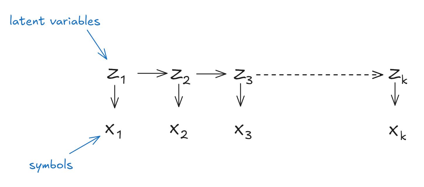
We model the joint distribution of the sequence as:
$$p(x) = p(x | z) p(z)$$
We model $p(x | z)$ as a Gaussian mixture model and use EM algorithm to estimate the parameters. We model $p(z)$ as a Markov chain and try to estimate the transition probabilities.
The intution behind this model is:
- The model was usually used for speech modeling.
- Humans also think something in their brain which is not observable just like the latent variables and emit sounds which are observable just like the symbols.
Recurrent Neural Networks
The problem with HMMs was that the length of the input sequence was always fixed.
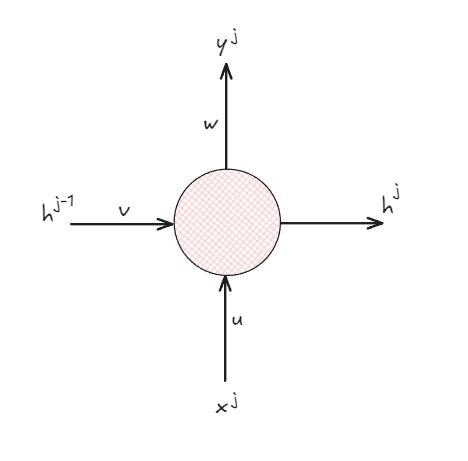
- $h^j = \sigma(vh^{j-1} + \alpha x^j + b)$ is the hidden state at time $j$
- $y^j = \sigma(wh^j + b’)$ is the output at time $j$
RNN were able to handle variable length inputs by sharing parameters across time and were able to be used as language models.
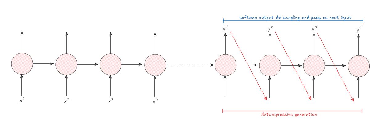
We train such models using cross entropy loss by doing ERM with gradient descent. The main problem with RNNs was that we had to pass each token one by one and could not parallelize the computation.
At the same time Unet architectures with skip connections were becoming popular in CV. We can use the same idea in NLP.
Transformers
Attention head
Transformers can be seen as RNNs with skip connections flipped 90 degrees.
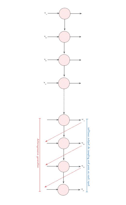
Lets consider we have just 1 data point consisting of $k$ tokens $x = { x^1, x^2, \ldots, x^k }$ We define 3 learnable matrices $W_q, W_k, W_v$ defined as:
- $q^j = W_q x^j$ is called the query vector
- $k^j = W_k x^j$ is called the key vector
- $v^j = W_v x^j$ is called the value vector
There is a latent/hidden vector $z^j$ for each token $x^j$ calculated as:
$$z^j = \sum_{t=1}^{m} \alpha_{j}^{t} v^{t}$$
where $\alpha_{j}^{t}$ is a measure of how much attention the token $x^j$ pays to the token $x^t$ and is calculated by just taking the dot product of the query vector:
$$\alpha_{j}^{t} = (q^j)^T k^t$$
However, we scale down the dot product by $\sqrt{d}$ to prevent it from exploding where $d$ is the dimension of the key and query vectors.
Also, we take a softmax of the attention scores to ensure that they sum to 1. hence usually you will find the following in the literature:
$$\alpha_{j}^{t} = \text{softmax}\left( \frac{(q^j)^T k^t}{\sqrt{d}} \right)$$
A good way to think of attention is to think of it as projecting every token to a new space that is a function of all the tokens.
We can concatenate all the tokens into matrices $Q = [q^1, q^2, \ldots, q^k]$, $K = [k^1, k^2, \ldots, k^k]$, and $V = [v^1, v^2, \ldots, v^k]$ to compute attention for all tokens in parallel using matrix multiplication:
$$Z = V \cdot \text{softmax}\left(\frac{Q^T K}{\sqrt{d}}\right)$$
Multi-head attention
Just like we have multiple kernels in CNNs, we can have multiple attention heads. To get multihead attention, say $h$ heads, we concatenate the outputs $Z_1, Z_2, \ldots, Z_h$ from each attention head and project it using a learnable matrix $W_o$ to get the final output:
$$Z = W_o[Z_1; Z_2; \ldots; Z_h]$$